Task 1: Modeling
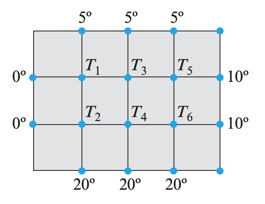
The figure below shows a metal plate whose edges are held at the temperatures shown. It follows from thermodynamic principles that the temperature at each of the six interior nodes will eventually stabilize at a value that is approximately the average of the temperatures at the four neighboring nodes. These are called the steady-state temperatures at the nodes.
Find a linear system whose solution gives the steady-state temperatures at the nodes, and use scipy to solve that system.
Task 2: Linear Programming by Affine Scaling
Implement in python the affine-scaling method and solve the following problem:
\[\begin{array}{rl} \max\;& z=x_1+2x_2\\ &x_1+x_2\leq 8\\ &x_1\geq 0,x_2\geq 0 \end{array}\]It is the same problem as seen in the slides. But now solve it assuming the starting solution is $[x_1, x_2]=[1, 3]$. The optimal solution is $[0,8]$.
You can then solve also the following problem:
\[\begin{array}{rl} \text{maximize} \;\;&2x_1 + 3x_2 + 2x_3 \\ \text{subject to} \; \; &x_1 + x_2 +2x_3 = 3\\ &x_1,x_2,x_3 \geq 0. \end{array}\]using as starting solution $[x_1, x_2, x_3]=[1, 3/2, 1/4]$.
How should the algorithm change if the problem was a minimization problem?
Solution:# %%
from fractions import Fraction
import numpy as np
np.set_printoptions(precision=3, suppress=True)
# %%
def affine_scaling(c, A, b, x_0, alpha=0.5):
x = x_0
x_old=np.zeros(len(x))
while np.linalg.norm(x_old-x)>0.001:
x_old=x
D=np.diag(x)
D1=np.linalg.inv(D)
x_tilde = D1 @ x
A_tilde = A @ D
c_tilde = c @ D
P=np.identity(len(x))-A_tilde.T @ np.linalg.inv( A_tilde @ A_tilde.T) @ A_tilde
p_tilde=P @ c_tilde
theta = np.max([abs(v) for v in p_tilde if v<0])
x_tilde = x_tilde + alpha/theta * p_tilde
x = D @ x_tilde
print(x)
return x
# %%
c = np.array([1, 2, 0])
A = np.array([[1, 1, 1]])
b = np.array([8])
x_0=np.array([1,3,4])
alpha = 0.5
affine_scaling(c, A, b, x_0, alpha)
# %%
c = np.array([2, 3, 2])
A = np.array([[1, 1, 2]])
b = np.array([3])
x_0=np.array([1, 3/2, 1/4])
alpha = 0.5
affine_scaling(c, A, b, x_0, alpha)
# %%
c = np.array([5, 4, 3, 0, 0, 0])
A = np.array([[2, 3, 1, 1, 0, 0],
[4, 1, 2, 0, 1, 0],
[3, 4, 2, 0, 0, 1],
])
b = np.array([5, 11, 8])
x_0=np.array([0.5, 1, 0.5, 0.5, 7, 1.5])
alpha = 0.5
affine_scaling(c, A, b, x_0, alpha)[1.046 4.954 2. ]
[0.934 6.066 1. ]
[0.724 6.776 0.5 ]
[0.465 7.285 0.25 ]
[0.249 7.626 0.125]
[0.125 7.812 0.062]
[0.063 7.906 0.031]
[0.031 7.953 0.016]
[0.016 7.977 0.008]
[0.008 7.988 0.004]
[0.004 7.994 0.002]
[0.002 7.997 0.001]
[0.001 7.999 0. ]
[0. 7.999 0. ]
[0.636 2.114 0.125]
[0.318 2.536 0.073]
[0.159 2.763 0.039]
[0.08 2.881 0.02 ]
[0.04 2.94 0.01]
[0.02 2.97 0.005]
[0.01 2.985 0.002]
[0.005 2.993 0.001]
[0.002 2.996 0.001]
[0.001 2.998 0. ]
[0.001 2.999 0. ]
[0. 3. 0.]
[0.96 0.672 0.815 0.25 4.86 0.804]
[1.38 0.336 1.005 0.226 3.133 0.505]
[1.604 0.168 1.088 0.199 2.238 0.339]
[1.724 0.084 1.142 0.159 1.738 0.209]
[1.809 0.042 1.147 0.11 1.431 0.113]
[1.888 0.021 1.096 0.064 1.233 0.059]
[1.945 0.01 1.046 0.032 1.117 0.03 ]
[1.973 0.005 1.022 0.016 1.059 0.016]
[1.987 0.003 1.011 0.008 1.029 0.008]
[1.993 0.001 1.005 0.004 1.015 0.004]
[1.997 0.001 1.003 0.002 1.007 0.002]
[1.998 0. 1.001 0.001 1.004 0.001]
[1.999 0. 1.001 0.001 1.002 0.001]
[2. 0. 1. 0. 1.001 0. ]
[2. 0. 1. 0. 1. 0.]
array([2., 0., 1., 0., 1., 0.])Task 3: Linear Programming for Project Selection
Model in linear programming terms the following problem: Given a set of projects to invest on, each with a cost and an expected profit, determine which to include in a collection so that the total cost is less than or equal to a given budget and the total expected profit is as large as possible. Reason about the nature of the variables, continuous or discrete.
Solve the instance of the problem given in the python code below in two ways:
-
with
scipy.optimization.linprogfrom the latest versions of scipy, -
with your implementation of the Affine Scaling method seen in the lecture.
The previous solution methods will only solve the continuous variables case. It is anyway a good exercise to solve the problem with continuous variables and then try to derive an integer solution from the fractional one. How would you do?
import numpy as np

num_items=100
capacity=997
profit = np.array([585, 194, 426, 606, 348, 516, 521, 1092, 422, 749, 895, 337, 143, 557, 945, 915, 1055, 546, 352, 522, 109, 891, 1001, 459, 222, 767, 194, 698, 838, 107, 674, 644, 815, 434, 982, 866, 467, 1094, 1084, 993, 399, 733, 533, 231, 782, 528, 172, 800, 974, 717, 238, 974, 956, 820, 245, 519, 1095, 894, 629, 296, 299, 1097, 377, 216, 197, 1008, 819, 639, 342, 807, 207, 669, 222, 637, 170, 1031, 198, 826, 700, 587, 745, 872, 367, 613, 1072, 181, 995, 1043, 313, 158, 848, 403, 587, 864, 1023, 636, 129, 824, 774, 889])
cost = np.array([485, 94, 326, 506, 248, 416, 421, 992, 322, 649, 795, 237, 43, 457, 845, 815, 955, 446, 252, 422, 9, 791, 901, 359, 122, 667, 94, 598, 738, 7, 574, 544, 715, 334, 882, 766, 367, 994, 984, 893, 299, 633, 433, 131, 682, 428, 72, 700, 874, 617, 138, 874, 856, 720, 145, 419, 995, 794, 529, 196, 199, 997, 277, 116, 97, 908, 719, 539, 242, 707, 107, 569, 122, 537, 70, 931, 98, 726, 600, 487, 645, 772, 267, 513, 972, 81, 895, 943, 213, 58, 748, 303, 487, 764, 923, 536, 29, 724, 674, 789])
# %%
from scipy.optimize import linprog
import numpy as np

# %%
num_items=100
capacity=997
profit = np.array([585, 194, 426, 606, 348, 516, 521, 1092, 422, 749, 895, 337, 143, 557, 945, 915, 1055, 546, 352, 522, 109, 891, 1001, 459, 222, 767, 194, 698, 838, 107, 674, 644, 815, 434, 982, 866, 467, 1094, 1084, 993, 399, 733, 533, 231, 782, 528, 172, 800, 974, 717, 238, 974, 956, 820, 245, 519, 1095, 894, 629, 296, 299, 1097, 377, 216, 197, 1008, 819, 639, 342, 807, 207, 669, 222, 637, 170, 1031, 198, 826, 700, 587, 745, 872, 367, 613, 1072, 181, 995, 1043, 313, 158, 848, 403, 587, 864, 1023, 636, 129, 824, 774, 889])
cost = np.array([[485, 94, 326, 506, 248, 416, 421, 992, 322, 649, 795, 237, 43, 457, 845, 815, 955, 446, 252, 422, 9, 791, 901, 359, 122, 667, 94, 598, 738, 7, 574, 544, 715, 334, 882, 766, 367, 994, 984, 893, 299, 633, 433, 131, 682, 428, 72, 700, 874, 617, 138, 874, 856, 720, 145, 419, 995, 794, 529, 196, 199, 997, 277, 116, 97, 908, 719, 539, 242, 707, 107, 569, 122, 537, 70, 931, 98, 726, 600, 487, 645, 772, 267, 513, 972, 81, 895, 943, 213, 58, 748, 303, 487, 764, 923, 536, 29, 724, 674, 789]])


# %%
sol=linprog(c=-profit, A_ub=cost, b_ub=997, bound=(0,1), integrality=0)

print(sol.x)
print(sol.x @ profit)
# %%15239.857191091372Task 4
Consider the following LP problem:
\[\begin{align*} \max \quad &5x_1 + 4x_2 + 3x_3 \\ \text{s.t.} \quad &2x_1 + 3x_2 + x_3 \leq 5 \\ &4x_1 + x_2 + 2x_3 \leq 11 \\ &3x_1 + 4x_2 + 2x_3 \leq 8 \\ &x_1,x_2,x_3 \geq 0 \end{align*}\]and an initial solution $\vec x = \begin{bmatrix} 0.5, 1, 0.5\end{bmatrix}$. Solve the problem with the Affine Scaling method.
Task 5
Show that if $A$ is a square matrix that can be reduced to a row echelon form $U$ by Gaussian elimination without row interchanges, then $A$ can be factored as $A = LU$, where $L$ is a lower triangular matrix.
Show that the LU decomposition can be rewritten as
\[A=LDU\]where now both the lower triangular factor and the upper triangular factor have 1’s on the main diagonal.
Solution: We know that the Gaussian elimination operations can be accomplished by multiplying $A$ on the left by an appropriate sequence of elementary matrices; that is, there exist elementary matrices $E_1,E_2,...,E_k$ such that $$ E_k \cdots E_2E_1A = U' $$ where U' is an upper triangular matrix with entries equal to 1 in the diagonal. Since elementary matrices are invertible, we can solve for $A$ as $$ A = E_1^{-1}E_2^{-1} \cdots E_k^{-1}U $$ $$ A = LU' $$ $$ L = E_1^{-1}E_2^{-1} \cdots E_k^{-1} $$ $L$ is lower triangular because: i) multiplying a row by a nonzero constant, and adding a scalar multiple of one row to another generate elementary matrices that are lower triangular. ii) multiplication of lower traingular matrices preserves the lower triangular property iii) inverse of lower traingular matrices preserves the lower triangular property.To show that the $LU'$ decomposition can be rewritten as $$ A=L'DU' $$ we just ``shift'' the diagonal entries of $L$ to a diagonal matrix $D$ and write $L$ as $L' = LD'$. In general, $LU$-decompositions are not unique. $$ A=LU= \begin{bmatrix} l_{11}& 0 &0 \\ l_{21}& l_{22}& 0 \\ l_{31}& l_{32}& l_{33}\\ \end{bmatrix} \begin{bmatrix} 1 &u_{12} &u_{13}\\ 0 &1 &u_{23}\\ 0 &0 &1\\ \end{bmatrix} $$ and $L$ has nonzero diagonal entries (which will be true if $A$ is invertible), then we can shift the diagonal entries from the left factor to the right factor by writing $$ \begin{array}{rl} A=& \begin{bmatrix} 1 &0&0\\ l_{21}/l_{11}& 1& 0\\ l_{31}/l_{11} &l_{32}/l_{22}& 1 \end{bmatrix} \begin{bmatrix} l_{11}&0&0\\ 0& l_{22} &0 \\ 0 &0& l_{33} \end{bmatrix} \begin{bmatrix} 1&u_{12}&u_{13}\\ 0& 1 &u_{23}\\ 0 &0 &1 \end{bmatrix} \\ = & \begin{bmatrix} 1& 0& 0\\ l_{21}/l_{11}& 1 &0\\ l_{31}/l_{11}& l_{32}/l_{22}&1\\ \end{bmatrix} \begin{bmatrix} l_{11} &l_{11}u_{12}& l_{11}u_{13}\\ 0& l_{22}& l_{22}u_{23}\\ 0 &0 &l_{33}\\ \end{bmatrix} \end{array} $$ which is another LU-decomposition of $A$.
Task 6
Propose an efficient method for solving $Ax=b$ and $A^T\tilde{x}=\tilde{b}$.
Solution: Find $A = PLU$. Then solve: $$ \vec z_1 = P^T \vec b, \qquad \qquad \vec L\vec z_2 = \vec z_1, \qquad \qquad U\vec x = \vec z_2 $$Task 7
Find the LU decomposition of the matrix
\[A=\begin{bmatrix} 3 &−6 &−3 \\ 2 &0 &6 \\ −4 &7 &4 \end{bmatrix}.\]Using the decomposition:
- solve the system of linear equations: $Ax=b$ when $b=[-3, -22, 3]$
- find the inverse of $A$.
Task 8
Software libraries vary in how they handle LU-decompositions. For example, many libraries perform row interchanges to reduce roundoff error and hence produce PLU-decompositions, even when asked for LU-decompositions. Find out which function(s) performs the LU-decomposition in Python Scipy and see what happens when you use scipy to find an LU-decomposition of the matrix from the previous task. (Hint: compare scipy.linalg.lu, scipy.linalg.lu_factor, scipy.linalg.lu_solve, scipy.sparse.linalg.splu). Update your implementation of Task 1 such that it does not need to compute any matrix inversion.
Task 9
Show that if $A$ is a real-valued symmetric (hence square) positive definite matrix, then $A$ can be factored as $A = LL^T$, where $L$ is a lower triangular matrix and $L$ is unique.
Show that the Cholseky decomposition can be rewritten as
\[A=LDL^T\]where now the diagonal elements of $L$ are required to be 1 and $D$ is a diagonal matrix.
Task 10
Propose an efficient method for solving $Ax=b$ where $A$ is a real-valued symmetric positive definite matrix.
The system: $$LL^Tx=b$$ can be solved by first solving $$Lw=b$$ and then solving: $$L^Tx=w$$ The latter two systems are easy to compute because the matrices are triangular. Overall it taks $O(n)$ instead of $O(n^3)$ of the Gaussian elimination.Task 11
Test whether the following martix is positive definite:
\[A=\begin{bmatrix} 3 &2 &−4 \\ 2 &0 &7 \\ −4 &7 &4 \end{bmatrix}.\]If it is not, generate a positive definite matrix from it and find its $LL^T$ decomposition. Using the decomposition:
- solve the system of linear equations: $Ax=b$ when $b=[-3, -22, 3]$
- find the inverse of $A$.
Task 12
Find out which function(s) performs the Cholseky decomposition in Python Scipy and see what happens when you use scipy to find a Cholesky decomposition of the matrix from the previous task. (Hint: compare scipy.linalg.cholesky, scipy.linalg.cho_factor, scipy.linalg.cho_solve.)
Task 13
Update the Affine Scaling algorithm above to use the Cholesky decomposition and resolve the LP problems above.
# %%
import numpy as np
import scipy as sp
import scipy.linalg as spla

np.set_printoptions(precision=3, suppress=True)


# %%
A = np.array([
    [3,2,-4],
    [2, 0, 7],
    [-4, 7,4]
    ])

AA = A @ A.T

print(AA)

L=spla.cholesky(AA, lower=True)

print(L)
print(np.allclose(AA, L @ L.T))

print(spla.cho_factor(AA))

# %%

def affine_scaling_cho(c, A, b, x_0, alpha=0.5):
    x = x_0
    x_old=np.zeros(len(x))

    while np.linalg.norm(x_old-x, ord=2)>0.001:
        x_old=x
        D=np.diag(x)
        D1=np.linalg.inv(D)

        x_tilde = D1 @ x
        A_tilde = A @ D
        c_tilde = c @ D

        v=A_tilde @ c_tilde
        AA = A_tilde @ A_tilde.T

        if True:
            ## solve AA^T w = v
            L = spla.cholesky(AA, lower=True)
            ## LL^T w = v
            ## Ly=v
            ## L^Tw=y
            y = spla.solve_triangular(L, v, lower = True)
            w = spla.solve_triangular(L.T, y, lower = False)
        else:
            L, low = spla.cho_factor(AA)
            w = spla.cho_solve((L, low), v)

        p_tilde = c_tilde - A_tilde.T @ w

        theta = np.max([abs(v) for v in p_tilde if v<0])

        x_tilde = x_tilde + alpha/theta * p_tilde
        x = D @ x_tilde
        print(x)
    return x

# %%

c = np.array([5, 4, 3, 0, 0, 0])
A = np.array([[2, 3, 1, 1, 0, 0],
            [4, 1, 2, 0, 1, 0],
            [3, 4, 2, 0, 0, 1],
            ])
b = np.array([5, 11, 8])

x_0=np.array([0.5, 1, 0.5, 0.5, 7, 1.5])
alpha = 0.5

affine_scaling_cho(c, A, b, x_0, alpha)
# %%
[[ 29 -22 -14]
[-22 53 20]
[-14 20 81]]
[[ 5.38516481 0. 0. ]
[-4.08529744 6.02580657 0. ]
[-2.59973473 1.55652363 8.47458633]]
True
(array([[ 5.38516481, -4.08529744, -2.59973473],
[-22. , 6.02580657, 1.55652363],
[-14. , 20. , 8.47458633]]), False)
[0.96 0.672 0.815 0.25 4.86 0.804]
[1.38 0.336 1.005 0.226 3.133 0.505]
[1.604 0.168 1.088 0.199 2.238 0.339]
[1.724 0.084 1.142 0.159 1.738 0.209]
[1.809 0.042 1.147 0.11 1.431 0.113]
[1.888 0.021 1.096 0.064 1.233 0.059]
[1.945 0.01 1.046 0.032 1.117 0.03 ]
[1.973 0.005 1.022 0.016 1.059 0.016]
[1.987 0.003 1.011 0.008 1.029 0.008]
[1.993 0.001 1.005 0.004 1.015 0.004]
[1.997 0.001 1.003 0.002 1.007 0.002]
[1.998 0. 1.001 0.001 1.004 0.001]
[1.999 0. 1.001 0.001 1.002 0.001]
[2. 0. 1. 0. 1.001 0. ]
[2. 0. 1. 0. 1. 0.]
array([2., 0., 1., 0., 1., 0.])