Task 1
Show that for an $n\times n$ matrix $E$ whose columns are the vectors of an orthonormal basis $E^{-1}=E^T$.
Task 2
Show that for any $m\times n$ matrix $A$, $AA^T$ is a symmetric matrix of size $m\times m$ and $A^TA$ is a symmetric matrix of size $n\times n$.
Task 3
Show that a real matrix is symmetric if and only if it is orthogonally diagonalizable.
Task 4 - PCA Visually
Consider 100 students with Physics and Statistics grades shown in the two diagrams below.
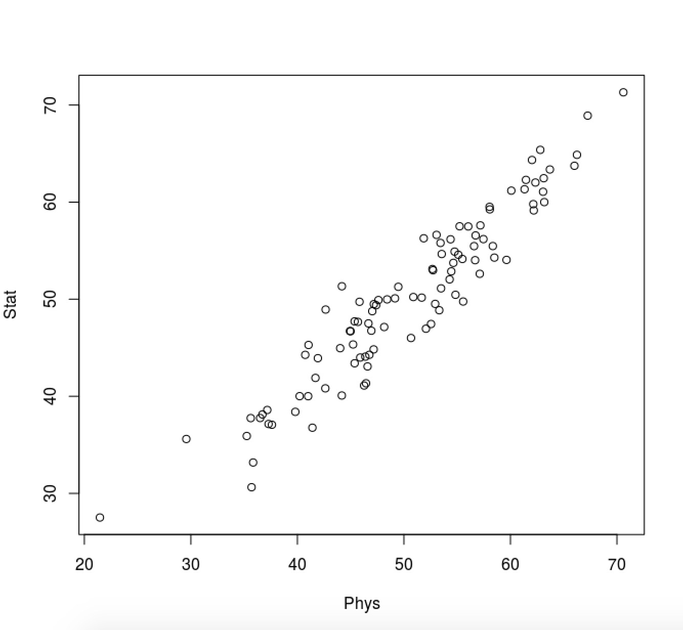
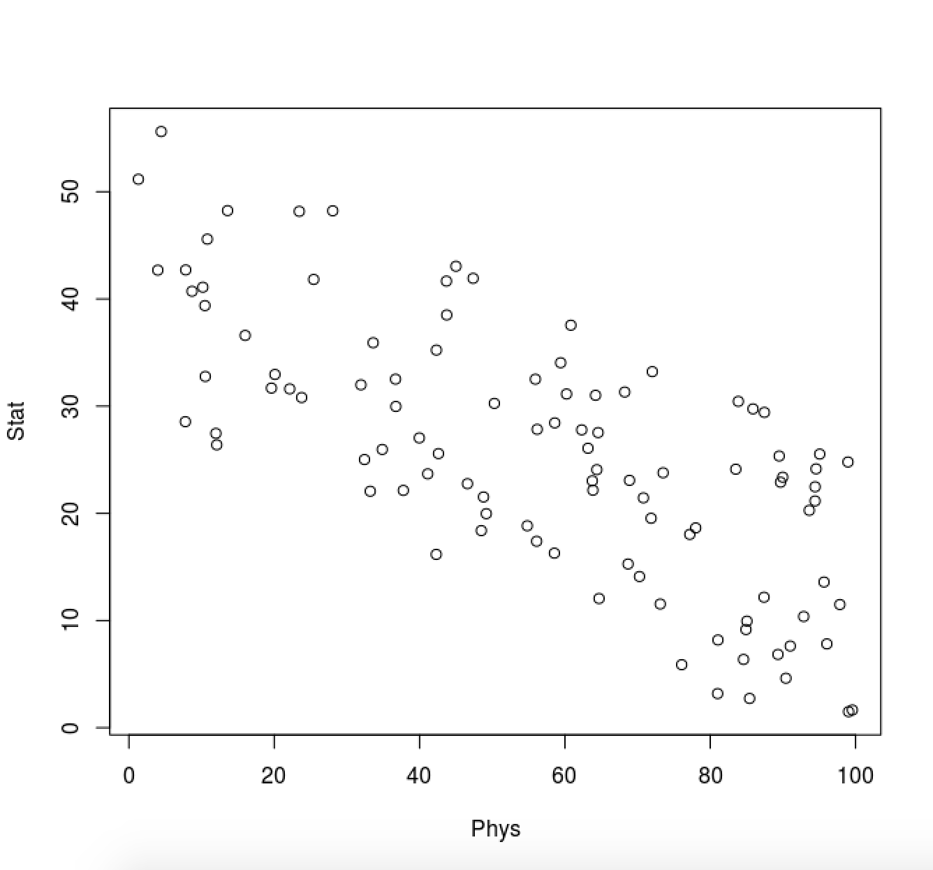
For each diagram:
-
Which is the direction (as a vector) along which the data varies the most?
-
What is (roughly) the point representing the mean value of the statistics/mathematics degree?
Task 5 - Covariance Matrix
Assume the following grades:
    Student   Math   English   Art
  --------- ------ --------- -----
          1     90        60    90
          2     90        90    30
          3     60        60    60
          4     60        60    90
5 30 30 30-
Define a matrix $X’$ where the rows represent samples (students), and the columns represent features (the different tests).
-
Perform mean centering: subtract each data value from its variable’s measured mean so that its empirical mean (average) is zero, call the resulting matrix $X$.
-
Without computing, what do you expect the covariance between a) Math and English and b) English and Art to be? Postive or negative?
-
Ignoring Bessel’s correction, which formula must be used to compute the covariance matrix?
-
Compute the variance of each test grades and the covariance between the test grades.
-
Determine the covariance matrix a) with Bessel’s correction, b) without Bessel’s correction.
Task 6 - Projection onto new feature space
When analysing the Iris dataset, we stored the data in form of a $150 \times 4$ matrix where the columns are the different features, and every row represents a separate flower sample. Let’s call this matrix $X$ and the first and the second principal component $w_1$ and $w_2$.
-
Using matrix multiplication, how do we project the 4-dimensional feature space onto a new 2-dimensional feature space that is spanned by $w_1$ and $w_2$? How does this relate to the formula on page 7 of the slide set?
-
Give the sizes of the matrices that you used in 1.)
Task 7 - Eigenfaces
In your git repository, beside the files needed for the assignment (helper.py and main.py) you find also the application EigenFace.py.
-
Run the script and download the images as described.
-
Run again the script. If all run smoothly you should be able to see the average images and a window with trackbars to change the weights of the principal components. Experiment with different values and observe the changes at the picture. Which characteristic of the image does each principl component captures?
-
After you have a working solution for the assignment you can uncommnet lines 141-149 and run the script again. Hovering on the window with the picture and pressing a key it is possible to iterate through the images and assess the distance of their PCA projection from the original image. Which face has the largest distance from its PC projection?
Task 8 - Eigenfaces
In your last mandatory assignment you will be using the PCA
functionality from OpenCV (https://opencv.org/). For this exercise, we
will use another set of tools, namely Google’s Colabatory framework
https://colab.research.google.com and, scikit-learn
(https://scikit-learn.org), a free software machine learning library
for Python for data analytics, statistics, machine learning, and Scipy
(https://www.scipy.org/, the scientific Python ecosystem). All of
those in itself can be quite overwhelming, however, the idea of this
exercise is to experience how easy it is to use and integrate all those.
Proceed as follows:
-
Download the Jupyter notebook
plot_eigenfaces.ipynbfrom here: https://scipy-lectures.org/packages/scikit-learn/auto_examples/plot_eigenfaces.html (at the very end of the page). -
Upload the notebook to https://colab.research.google.com.
-
Run the cells subsequently (you can safely ignore everything related to Support Vector classification, and anything after “Doing the Learning: Support Vector Machines”).
-
Add a cell (after cell 8) and print the vector in the 150-dimensional Eigenface-space that corresponds to the projection of the first image in the test dataset
X_test.